
FastSpeech 2 and 2s: Fast, High-Quality, and Fully End-to-End TTS
Published:
FastSpeech 2 and 2s: Fast, High-Quality, and Fully End-to-End TTS
FastSpeech 2 is a non-autoregressive text-to-speech (TTS) model designed to simplify training, improve voice quality, and address the limitations of its predecessor FastSpeech. It eliminates the teacher-student training pipeline, introduces richer variance information (duration, pitch, and energy), and improves the alignment between text and speech. Building on this, FastSpeech 2s extends the architecture to support fully end-to-end text-to-waveform synthesis, skipping the intermediate mel-spectrogram generation altogether. Listen to audio samples —
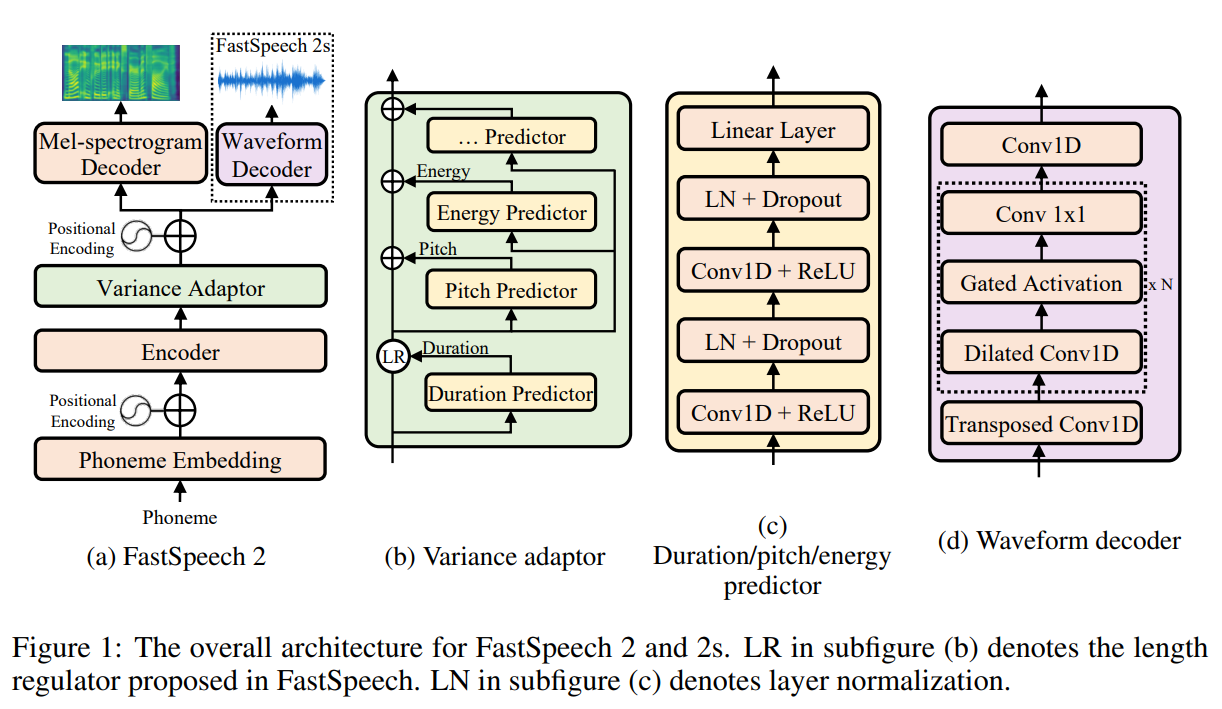
The model consists of an encoder that processes phoneme embeddings, followed by a variance adaptor module that incorporates duration, pitch, and energy information via corresponding predictors. The length regulator expands encoder outputs based on predicted durations. Pitch and energy predictors generate continuous features, which are quantized and embedded before being added to the decoder input. The decoder generates the mel-spectrogram, which is then converted to waveform by a neural vocoder during inference. All predictors are trained with explicit supervision from extracted ground-truth values.
1. Motivation
FastSpeech 2 was motivated by key shortcomings in FastSpeech:
- Autoregressive reliance for supervision: FastSpeech used a teacher model to guide learning, introducing unnecessary complexity.
- Imperfect duration alignment: Duration extracted from autoregressive attention maps was often inaccurate.
- Information loss from knowledge distillation: Mel-spectrograms from the teacher model lacked pitch, energy, and other prosodic nuances.
The One-to-Many Mapping Problem in TTS
A single text sequence can correspond to multiple plausible speech outputs due to natural variation in duration, pitch, energy, and prosody. Without explicit modeling of these variations, non-autoregressive models tend to overfit or generalize poorly. FastSpeech 2 addresses this by directly supervising the model with ground-truth targets and explicit variance features.
2. Model Overview
The FastSpeech 2 architecture is composed of:
- Phoneme Embedding Layer: Converts text (converted to phonemes) into embeddings.
- Encoder: A stack of Feed-Forward Transformer (FFT) blocks that processes phoneme embeddings.
- Variance Adaptor: Injects prosodic and acoustic features (duration, pitch, energy) into the hidden representation.
- Mel-Spectrogram Decoder: Converts the variance-adapted sequence into mel-spectrograms in parallel.
- Waveform Decoder (FastSpeech 2s): Directly generates raw audio from the adapted sequence.
Positional encodings are applied at both encoder and decoder ends.
3. Variance Adaptor: Modeling Duration, Pitch, and Energy
3.1 Duration Predictor
- A major challenge in non-autoregressive TTS is aligning discrete phoneme tokens to continuous mel-spectrogram frames.
- FastSpeech 2 addresses this by introducing a duration predictor that explicitly estimates the number of frames each phoneme should span.
- Instead of relying on alignment learned from an autoregressive teacher model (as in FastSpeech-1), FastSpeech 2 uses Montreal Forced Aligner (MFA) tool to extract ground-truth phoneme durations(phoneme boundary error reduced from 19.68 ms to 12.47 ms).
- The predictor operates on the phoneme hidden sequence produced by the encoder and forecasts the log-scale duration ℓ𝑖 = log(1+𝑑𝑖) for each phoneme 𝑖, where di is the frame count. (Logarithmic transformation stabilizes training by compressing dynamic ranges and encouraging Gaussian-like targets).
- The predicted durations are trained using a Mean Squared Error (MSE) loss.
- Length Regulator expands each encoder state ℎ 𝑖 to a sequence of length, effectively converting phoneme-level sequences into frame-level sequences suitable for spectrogram generation. (this is the length regulator proposed in FastSpeech-1).
3.2 Pitch(F₀) Predictor
- Directly predicting pitch contours in the time domain is challenging due to their high temporal variability and non-Gaussian distribution.
- To overcome this, FastSpeech 2 models pitch in the frequency domain using the Continuous Wavelet Transform (CWT), which provides a multi-resolution representation of the pitch signal.
Continuous Wavelet Transform for Pitch
Given a continuous pitch contour function F₀(t), CWT converts it into a pitch spectrogram W(τ, t):
\[W(τ, t) = \frac{1}{\sqrt{τ}} \int_{-\infty}^{\infty} F₀(x) \, \psi\left(\frac{x - t}{τ}\right) \, dx\]Where:
- τ is the scale (related to frequency),
- ψ is the Mexican Hat wavelet,
- W(τ, t) captures pitch energy at different scales and time.
The original pitch contour can be reconstructed using inverse CWT:
\[F₀(t) = \sum_{i=1}^{K} \hat{W}_i(t) \cdot (i + 2.5)^{-5/2}\]with ( K = 10 ) components.
Predictor Architecture
- Operates on the length-regulated hidden sequence.
- Architecture:
- 2-layer 1D convolutional network (kernel size = 3)
- ReLU activation
- Layer normalization + dropout
- Linear layer → pitch spectrogram
- Final Linear layer projects to output dimension 𝐾 (CWT channels), yielding predicted pitch spectrogram
Training and Inference Workflow
Preprocessing:
- Extract F₀ using PyWorld Vocoder from the raw waveform.
- Interpolate unvoiced regions (where F₀ = 0) to create a continuous pitch contour.
- Convert F₀ to log-scale to stabilize numericals and compress dynamic ranges.
Compute the temporal mean (μ) and temporal standard deviation (σ) across the pitch contour:
\[\mu = \frac{1}{T} \sum_{t=1}^T \log F_0(t), \quad \sigma = \sqrt{ \frac{1}{T} \sum_{t=1}^T (\log F_0(t) - \mu)^2 }\]Normalize the log-scaled F₀ for a zero-mean, unit-variance contour:
\[F_0^{\text{norm}}(t) = \frac{\log F_0(t) - \mu}{\sigma}\]- Note: Normalization only affects the pitch prediction target, not the model input.
- Apply Continuous Wavelet Transform (CWT) to the normalized pitch to obtain the multi-scale pitch spectrogram \( W(\tau, t) \in \mathbb{R}^{K \times T} \), which is the target for pitch prediction.
- The computed utterance-level ground-truth \( \mu, \sigma \) is stored for training the mean and variance prediction branch.
Training:
- Spectrogram Prediction:
- Input: ( H )
Use Mean Squared Error (MSE): \(\mathcal{L}_{\text{pitch}} = \frac{1}{T} \sum_{t=1}^T \sum_{i=1}^{K} (\hat{W}_i(t) - W_i(t))^2\)
- Mean and Variance Prediction:
- Input: \( H \)
- Compute pooled vector: \(\bar{h} = \frac{1}{T} \sum_{t=1}^T h_t\)
- Pass \( \hat{\mu} \) through two independent linear layers:
These are trained using utterance-level MSE losses: \(\mathcal{L}_{\mu} = (\hat{\mu} - \mu)^2, \quad \mathcal{L}_{\sigma} = (\hat{\sigma} - \sigma)^2\)
Note: The predicted \( \hat{\mu} \) and \( \hat{\sigma} \) are not used in any model component during training, only evaluated for correctness against ground-truth. They are only used at inference time for pitch reconstruction.
Inference:
- Predict \( \hat{W}(\tau, t) \), \( \hat{\mu} \), \( \hat{\sigma} \) from text via encoder and pitch predictor.
- Apply inverse CWT to \( \hat{W} \) to reconstruct normalized pitch contour \( \hat{F}_0^{\text{norm}}(t) \).
- Denormalize using predicted stats: \(\hat{F}_0(t) = \hat{F}_0^{\text{norm}}(t) \cdot \hat{\sigma} + \hat{\mu}\)
- Quantize \( \hat{F}_0(t) \) to 256 log-scale bins.
- Embed each bin into a pitch embedding vector \( p_t \), and add to decoder input.
Benefits of CWT-based Modeling
- Improved pitch contour accuracy (closer σ, γ, kurtosis to real pitch).
- Lower DTW distance vs. ground-truth.
- CMOS improvement over direct pitch regression: +0.185 (FastSpeech 2).
- Enables fine-grained prosody control.
3.3 Energy Predictor
Energy Definition and Preprocessing
The ground-truth energy is computed per frame as the L2 norm of the Short-Time Fourier Transform (STFT) magnitude spectrum:
\[E_t = \left\| \text{STFT}_t \right\|_2 = \sqrt{ \sum_{f=1}^{F} |X_t(f)|^2 }\]Where:
- \( X_t(f) \) is the complex STFT magnitude at frame \( t \) and frequency bin \( f \),
- \( E_t \) is the scalar energy at time \( t \),
- This results in an energy contour \( E \in \mathbb{R}^{T} \), aligned with mel-spectrogram frames.
The energy contour is quantized into 256 uniformly spaced bins across the training set’s dynamic range, and each bin index is mapped to a trainable embedding vector.
These embeddings are used as additional inputs to the decoder during training, and predicted during inference.
Architecture
- The energy predictor shares the same CNN-based architecture as the pitch predictor:
- 2-layer 1D convolution (kernel size = 3, channel size = 256)
- ReLU activation
- Layer normalization + dropout
- Final Linear layer projects to a scalar energy value per frame: \( \hat{E}_t \)
- Operates on the length-regulated encoder hidden sequence \( H \in \mathbb{R}^{T \times d} \)
Training and Inference
Training:
Supervised regression using Mean Squared Error (MSE) between predicted and ground-truth energy:
\[\mathcal{L}_{\text{energy}} = \frac{1}{T} \sum_{t=1}^{T} (\hat{E}_t - E_t)^2\]During training, the quantized ground-truth energy bins are embedded and added to the decoder input.
Inference:
- Predict frame-level energy values \( \hat{E}_t \) using the energy predictor.
- Quantize \( \hat{E}_t \) into one of 256 bins.
- Lookup corresponding energy embedding vectors.
- Add embeddings to the decoder input sequence, alongside pitch and duration information.
3.4 Mel-Spectrogram Decoder (FastSpeech 2)
The mel-spectrogram decoder is responsible for generating a time-aligned mel-spectrogram from the prosody-conditioned hidden sequence output by the variance adaptor. It decodes frame-level hidden states into spectral frames, independently and in parallel, while preserving global context through self-attention.
Input Representation
The input to the mel-spectrogram decoder is a frame-level hidden sequence that combines:
- output of the Length Regulator
- pitch embeddings
- energy embeddings
- positional encoding added to inject temporal order into the sequence
All components are of shape \( \mathbb{R}^{T \times d} \), where \( T \) is the number of decoder time steps (aligned with mel frames), and \( d \) is the model dimension. They are added element-wise to form the final decoder input \( H’ \).
Positional Encoding:
Transformer architectures lack recurrence or convolution, so they require positional encodings to inject information about the position of each token in the sequence.
FastSpeech 2 adopts sinusoidal positional encodings as introduced in the original Transformer paper:
\[\text{PE}_{(t, 2i)} = \sin\left(\frac{t}{10000^{2i/d}}\right), \quad \text{PE}_{(t, 2i+1)} = \cos\left(\frac{t}{10000^{2i/d}}\right)\]These sinusoidal encodings:
- Are deterministic and require no learning
- Encode relative distance via linear combinations of sinusoids
- Allow the decoder to reason about both absolute and relative positions
In practice, \( PE \) is a tensor of shape \( \mathbb{R}^{T \times d} \), added element-wise to the variance-adapted sequence.
Why not learn positional encodings?
Learned encodings are an option, work well for shorter, fixed-length inputs, sinusoidal encodings generalize better to unseen sequence lengths a useful trait in TTS, because utterances can vary significantly in duration.
Architecture
The decoder consists of a stack of Feed-Forward Transformer (FFT) blocks, each containing:
- Multi-head self-attention:
- Enables every time step to attend to all others, modeling long-range dependencies
- Position-wise feed-forward network:
- Adds non-linearity and channel mixing
- Residual connections + Layer normalization:
- Improves gradient flow and stability
The number of FFT blocks (e.g., 6 layers) and the dimensionality (e.g., 256 or 384) can be adjusted based on the dataset and target latency. Since the model is non-causal, every output frame attends to both past and future context within the input sequence.
The decoder produces a mel-spectrogram:
\[\hat{S} = \text{Decoder}(H') \in \mathbb{R}^{T \times D}\]where \( D \) is the number of mel frequency channels (typically 80).
Output Conditioning
To improve reconstruction quality, the decoder may be followed by:
- Linear projection layer to map Transformer output to \( D \) mel channels
- Post-Net (optional): a 5-layer CNN that predicts a residual spectrogram to refine decoder output (originally used in Tacotron 2)
The output \( \hat{S} \) is used as input to the vocoder (e.g., Parallel WaveGAN) for waveform generation.
The decoder is trained using L1 reconstruction loss.
Inference
- The decoder operates in parallel across all time steps during inference.
- Unlike autoregressive models, it doesn’t rely on previous outputs, making it:
- More stable
- Faster
- Better aligned with input phoneme durations
The mel-spectrogram prediction is next passed to a vocoder for waveform.
4. FastSpeech 2s: Direct Text-to-Waveform Generation
FastSpeech 2s eliminates the FastSpeech 2’s vocoder (mel-spectrograms to waveforms) requirement by directly generating the waveform from the hidden representations.
4.1 Challenges in Direct Waveform Prediction
- High temporal resolution: Audio waveforms operate at 16k–24k Hz, resulting in extremely long sequences (thousands of samples per second).
- High information density: In addition to amplitude, waveform modeling requires capturing fine phase and harmonic structures.
- Long sequences exceed GPU limits: Processing full utterances is memory-intensive; training often relies on random waveform slices.
- Lack of global context: Sliced training limits the model’s ability to learn long-range coherence across the utterance.
4.2 Architecture
FastSpeech 2s adopts a WaveNet-inspired decoder to model waveform sequences directly. The key components are:
- Upsampling Network:
- Multiple transposed 1D convolution layers gradually upsample the encoder hidden sequence to match waveform resolution.
- Enables frame-to-sample alignment without losing contextual smoothness.
- Non-Causal Convolution Stack:
- Gated activations using tanh-sigmoid units.
- Dilated convolutions to capture long-range dependencies efficiently.
- 1x1 convolution layers for channel mixing and output projection.
- Output: Directly generates the raw waveform signal \( \hat{x}(t) \), eliminating the need for a spectrogram decoder or external neural vocoder.
4.3 Training Strategy
FastSpeech 2s is trained using a multi-component loss:
- Multi-resolution STFT Loss:
- Compares the magnitude spectra of predicted and ground-truth waveforms across multiple STFT window sizes and hop lengths.
- Captures both coarse and fine details of speech.
- Adversarial Loss (LSGAN):
- A Parallel WaveGAN-style discriminator is trained jointly.
- Uses least-squares GAN loss to ensure the generated waveform matches real speech in perceptual quality and phase structure.
Total Loss: \(\mathcal{L}_{\text{total}} = \lambda_{\text{STFT}} \cdot \mathcal{L}_{\text{STFT}} + \lambda_{\text{adv}} \cdot \mathcal{L}_{\text{adv}}\)
Typical values: \( \lambda_{\text{STFT}} = 1 \), \( \lambda_{\text{adv}} = 4 \)
4.4 Inference
- During inference, only the waveform decoder is used.
- The mel-spectrogram decoder is entirely discarded, making the model fully end-to-end from text to waveform.
- The model generates the waveform sample-by-sample (or chunk-wise), eliminating the need for any external vocoder like WaveGlow or HiFi-GAN.
5. Performance Evaluation
| Model | MOS Score | CMOS vs FS1 |
|---|---|---|
| Ground Truth | 4.30 ± 0.07 | — |
| Tacotron 2 (PWG) | 3.70 ± 0.08 | -0.885 |
| Transformer TTS | 3.72 ± 0.07 | -0.235 |
| FastSpeech | 3.68 ± 0.09 | 0.000 |
| FastSpeech 2 | 3.83 ± 0.08 | +0.000 |
| FastSpeech 2s | 3.71 ± 0.09 | — |
6. Efficiency
| Model | Training Time | Inference RTF | Speedup vs AR |
|---|---|---|---|
| Transformer TTS | 38.64h | 0.932 | 1.0× (baseline) |
| FastSpeech | 53.12h | 0.0192 | 48.5× |
| FastSpeech 2 | 17.02h | 0.0195 | 47.8× |
| FastSpeech 2s | — | 0.0180 | 51.8× |
7. Ablation Studies
| Setting | CMOS Drop |
|---|---|
| FastSpeech 2 | 0 |
| - without pitch | -0.245 |
| - without energy | -0.040 |
| - without pitch & energy | -0.370 |
| FastSpeech 2 - No CWT | -0.185 |
- Pitch modeling using CWT improves prosody.
- Energy and pitch significantly boost voice quality.
- The mel-spectrogram decoder is crucial even in FastSpeech 2s during training.
8. Variance Control
Because pitch, duration, and energy are explicitly modeled, FastSpeech 2 supports controllable synthesis:
- Adjusting pitch (e.g., F₀ = 0.75×, 1.0×, 1.5×) produces expected shifts in voice tone.
- This feature can be leveraged for emotion control, speaker adaptation, or style transfer.
9. Conclusion
FastSpeech 2 advances non-autoregressive TTS by:
- Eliminating the teacher-student pipeline
- Adding explicit variance modeling
- Improving prosody and robustness
- Enabling fast training and inference
FastSpeech 2s takes it further by generating waveform end-to-end. Both models demonstrate that high-quality speech synthesis can be fast, parallelizable, and controllable without autoregression.